4.7. Well Integrity

4.7.1. Description

The Well Integrity Monitoring application provides monitoring tools for well integrity in geothermal reservoirs: caliper log processing, remaining thickness on the schematic, corrosion-rate forecasting, annulus pressure monitoring, and Well Barrier Envelope (WBE) tracking.

4.7.2. Workflow (per Well Integrity Monitoring app)

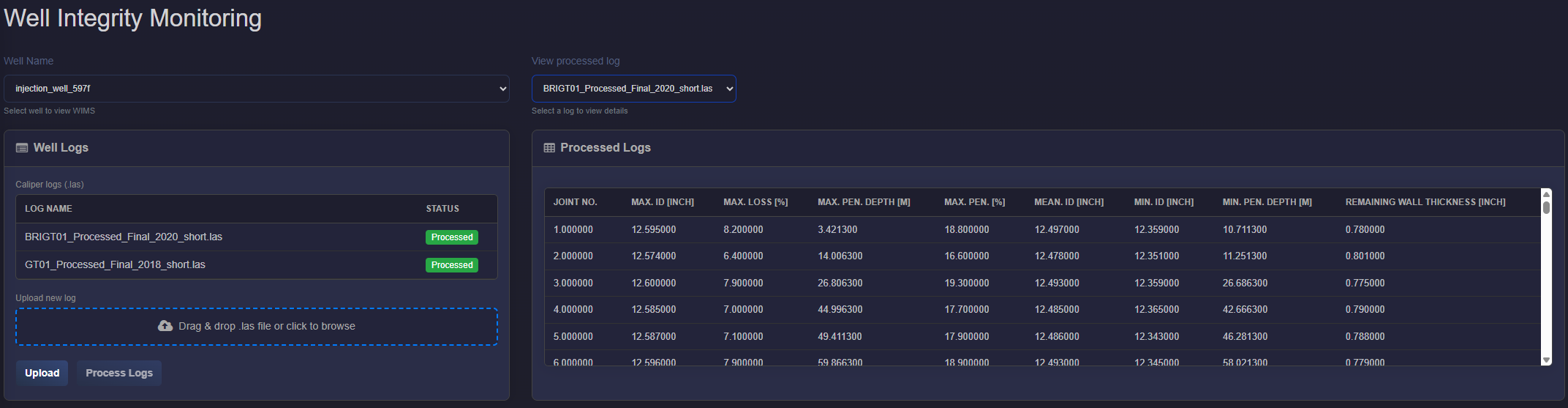
1. Select well — On opening the app, the plant is loaded. Choose Well Name from the dropdown to view WIMS for that well.

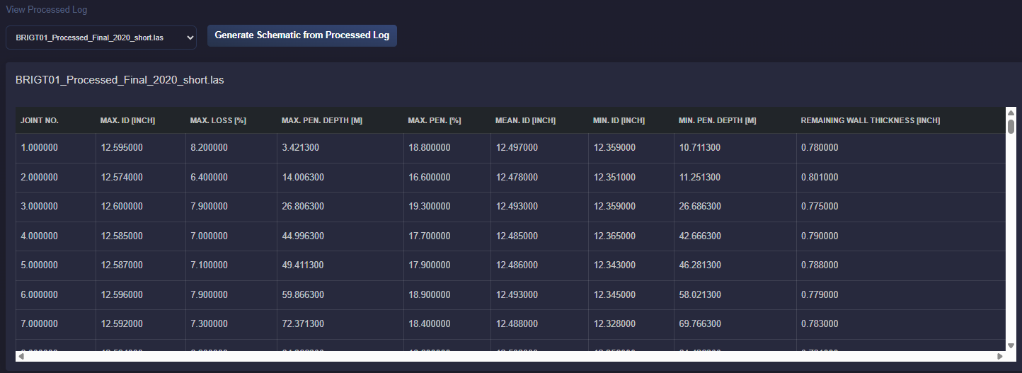
2. Upload and process caliper logs — In the Well Logs card (left): upload LAS caliper logs via drag‑and‑drop or Upload; click Process Logs to run processing. Processed logs appear in the table; select one in View processed log (right) to see the Processed Logs table (per‑joint ID, penetration, remaining thickness).

   

3. Well schematic — Create the well schematic in the Well Schematics application and ensure a well tally added in Well Parameters. The WIMS panel appears when the selected well has at least one saved schematic.

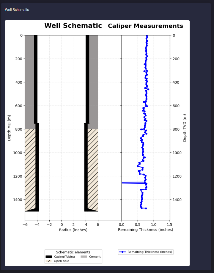
4. WIMS panel — Select a saved schematic in the WIMS card header; optionally click Save panel to store your configuration. The schematic image is shown (with remaining thickness overlay when a processed log is selected). Use the subcards:

   • Overall Integrity status — Last update date (date when the panel was last saved); status legend (Failed / Not verified / Verified).

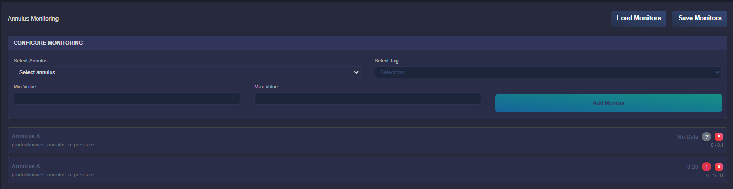
   • Annulus monitoring — Click Add monitor; in the modal choose the annulus (from the schematic), then Add. Each monitor is clickable: open it to Configure gauge (select Tag, set Min and Max value for alerts, or Delete monitor). Save the panel to persist monitors.

   • Well Barrier Envelope (WBE) — Click Add element; choose Primary or Secondary table, add from schematic or custom, and fill Qualification / Monitoring / Status / Remarks. Each barrier row is clickable: click to edit (Element, Qualification, Monitoring, Status, Remarks) or delete. Save panel to store.

   • WBE Risk — Click Add risk; fill Failure mode, Effect, Risk (Likelyhood‑Effect‑Risk Factor), Action Plan, Response time, Operate during failure. Each risk row is clickable to edit or delete. Save panel to store.

     

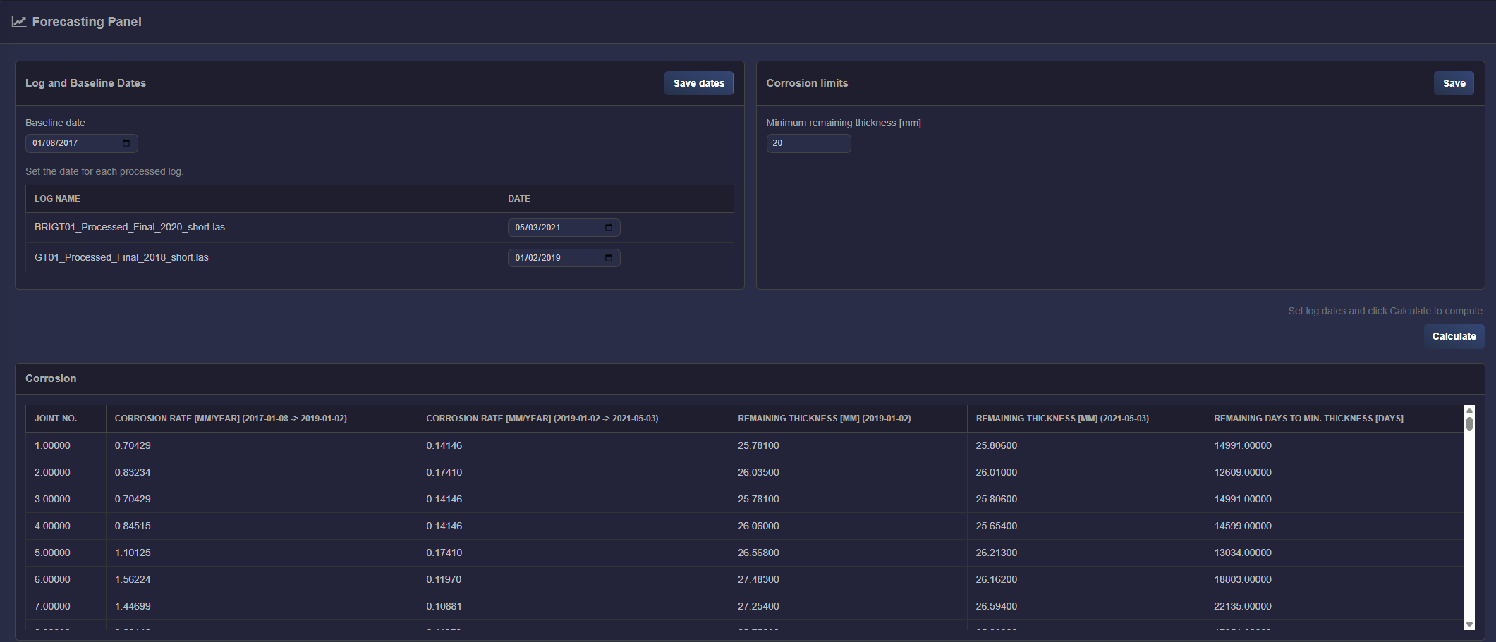
5. Forecasting Panel — In the Forecasting Panel: set Baseline date and a date for each processed log in Log and Baseline Dates, then click Save dates. Set Minimum remaining thickness [mm] in Corrosion limits and click Save. Click Calculate to compute corrosion rate and remaining days to min. thickness. The Corrosion table shows joint-wise corrosion rates, remaining thickness per log date, and remaining days to min. thickness.

   

4.7.3. Inputs

• Caliper log — LAS format (up to 2.0 supported). The file should have DATE or PID mnemonic for the logging date. Finger channels should be named D01, D02, etc. (double radii measurement).

• Well schematic — Created in the Well Schematics application; select a saved schematic in the WIMS panel.

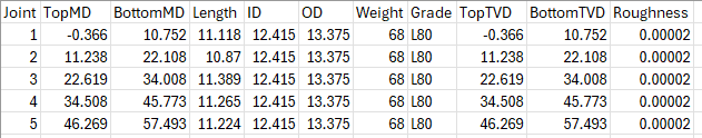
• Well tally — Required for joint-based processing. Provide via Well Parameters (app builder) . Format example:

  

4.7.4. Caliper log processing

Processing runs when you click Process Logs. For each well joint, the following are computed:

• Maximum, minimum and average ID

• Maximum loss percentage

• Maximum penetration and corresponding depth

• Minimum penetration and corresponding depth

• Remaining wall thickness (most pessimistic case)

Log depths should be calibrated to the same depth reference prior to processing.

4.7.5. WIMS panel (schematic and monitoring)

• Schematic — Select a saved schematic; the diagram is shown with optional remaining-thickness overlay when a processed log is selected.

• Overall Integrity status — Last update date; status legend: Failed (red), Not verified or other issues (amber), Verified and in good state (green).

• Annulus monitoring — Add monitors per annulus; configure Tag, Min value and Max value. Monitors can be saved with the panel. Data refresh: tag values (e.g. annulus pressure) are fetched from the application every 10 seconds for all configured monitors; the gauge display and min/max alerts update accordingly.

• Well Barrier Envelope (WBE) — Primary and Secondary barrier elements tables. Each row: Element, Qualification, Monitoring, Status (Failed / Not verified / Verified), Remarks. Add elements from schematic or as custom; edit or delete via row actions.

• WBE Risk — Table: Failure mode, Effect, Risk (Likelyhood‑Effect‑Risk Factor), Action Plan, Response time (months), Operate during failure. Add or edit risks via modals.

4.7.6. Forecasting panel

• Log and Baseline Dates — Baseline date (single date); table of log name and date for each processed log. Save dates stores them (used for corrosion-rate calculation).

• Corrosion limits — Minimum remaining thickness [mm]. Save stores the value (used for “remaining days to min. thickness”).

• Calculate — Enabled when Baseline date and all log dates are set. Computes corrosion rate between log intervals, remaining thickness at each log date, and (if minimum remaining thickness is set) remaining days until that minimum. Result table: Joint No., corrosion rate columns per interval, remaining thickness columns per log date, and “Remaining days to min. thickness [days]”.

4.7.6.1. Calculation logic (how the corrosion calculation is performed)

• Logs used — Only processed logs that have a date saved in Log and Baseline Dates are used. Logs are sorted chronologically by date (earliest first). The Baseline date is a single reference date (e.g. installation or first survey) and must be set.

• Corrosion rate [mm/year] — One column per time interval:

  • First interval (Baseline → first log): For each joint, ID at “baseline” is the nominal ID from the well tally (unchanged). ID at first log is the Min. ID from that processed log (worst case). Corrosion rate = | baseline ID − first‑log ID | in mm, divided by the time span (first log date − baseline date) in days, then × 365 to get mm/year.

  • Later intervals (consecutive log pairs): For each pair “previous log date → current log date”, ID is taken as Mean. ID from each processed log. Corrosion rate = | Mean. ID (previous) − Mean. ID (current) | in mm, divided by (current date − previous date) in days, then × 365 → mm/year.

  So with three logs (L1, L2, L3) you get: one column “Baseline → L1”, one “L1 → L2”, one “L2 → L3”. Each column is per joint; joints beyond the log length are left blank (NaN).

• Remaining thickness [mm] per log date — For each log (by date), for each joint: remaining thickness = (OD from well tally) − (Min. ID from that log), converted to mm (× 25.4). One column per log date: “Remaining thickness [mm] (YYYY-MM-DD)”.

• Remaining days to min. thickness — Uses the latest values only: the latest corrosion rate (the interval ending at the most recent log date) and the latest remaining thickness (at that most recent log date). For each joint: days = (remaining thickness [mm] − minimum remaining thickness [mm]) / (corrosion rate [mm/year]) × 365.25. If remaining thickness is already ≤ minimum, result is 0 days. If corrosion rate is ≤ 0 or missing, result is not defined (shown as blank). Values are rounded to whole days in the table.